

Download first → Sample Workbook – Dynamic Arrays Dashboard
TL;DR – Why You Should Care
- Dynamic arrays let one formula fill many cells (no Ctrl-Shift-Enter).
=FILTER()replaces clunky filter buttons.=UNIQUE()auto-de-dupes for data validation lists.=PIVOTBY()create pivot-style summaries in the grid.
Watch Them Spill
Here is a =FILTER() example in action.
And a =UNIQUE() example.
And finally a =PIVOTBY() example.
1 | Dynamic Arrays 101
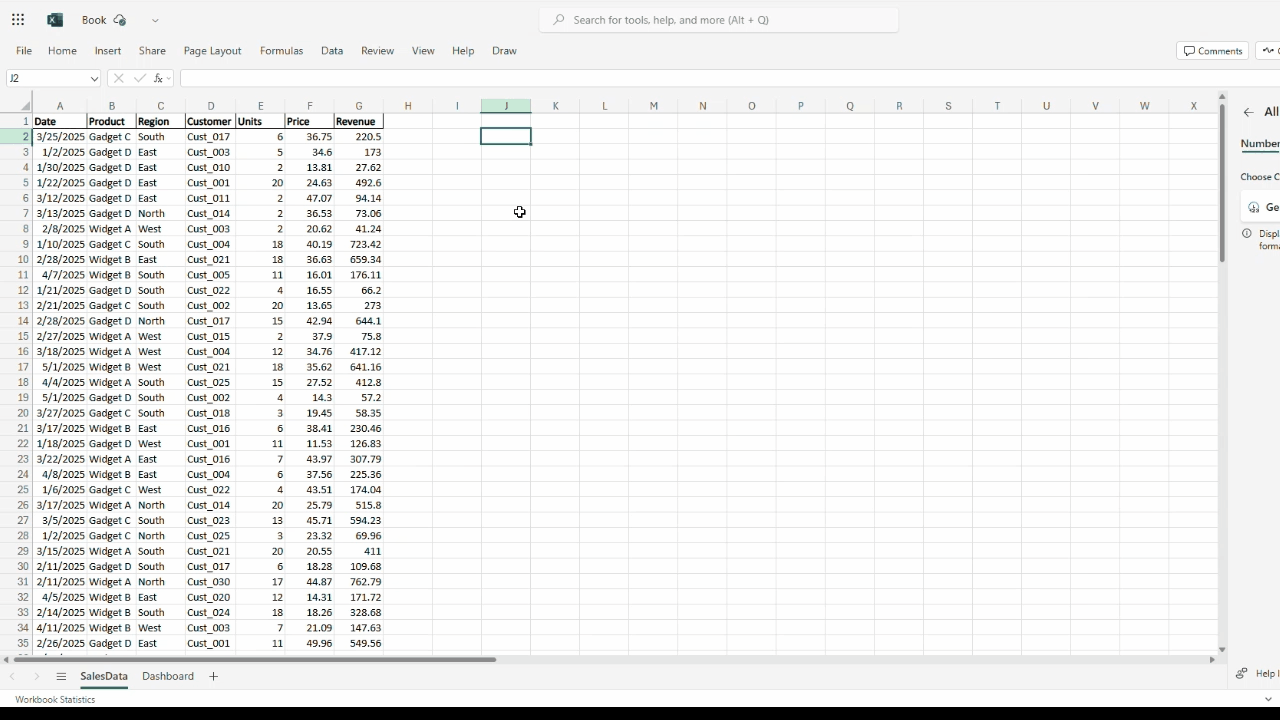
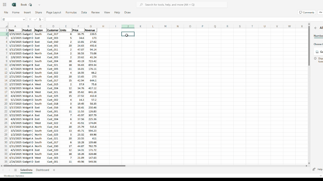
When a formula returns multiple values in Excel 365+, the extras spill into adjacent cells. Reference the entire range with a hash (B2#). If something blocks the spill, Excel shows #SPILL!—clear the blocker and carry on.
2 | The Core Six Functions
| Function | Why It Rocks | Quick Example |
|---|---|---|
| SEQUENCE | Create running numbers | =SEQUENCE(12) |
| RANDARRAY | Random sampling | =RANDARRAY(5,1,0,1,TRUE) |
| UNIQUE | De-dupe lists | =UNIQUE(SalesData[Customer]) |
| SORT / SORTBY | Alphabetize or custom order | =SORTBY(A2:B10,B2:B10,-1) |
| FILTER | SQL-style WHERE clause | =FILTER(Table1,Table1[Region]="West") |
| XLOOKUP | Spill-friendly lookup | =XLOOKUP(ProductList,PriceTable[Product],PriceTable[Price]) |
3 | 2023-25 Power-Ups
| New Function | Elevator Pitch | Tiny Demo |
|---|---|---|
| TAKE / DROP | Slice rows/cols from top/bottom | =TAKE(A2:F100,-5) |
| CHOOSEROWS / CHOOSECOLS | Select arbitrary rows/cols | =CHOOSECOLS(Data,1,4,7) |
| VSTACK / HSTACK | Append tables | =VSTACK(Jan#,Feb#) |
| EXPAND | Pad spills to fixed size | =EXPAND(B2#,10,5,"") |
| GROUPBY | One-axis summary | =GROUPBY(Table[Date],YEAR(Table[Date]),"Rev",SUM(Table[Revenue])) |
| PIVOTBY | Two-axis pivot | =PIVOTBY(Table[Region],Table[Product],Table[Revenue],SUM) |
4 | Hands-On: Build an Auto-Updating Sales Dashboard
- Current-month orders:
=FILTER(SalesData, MONTH(SalesData[Date]) = MONTH(TODAY())) - Unique customers:
=COUNTA(UNIQUE(FILTER(SalesData[Customer], MONTH(SalesData[Date]) = MONTH(TODAY())))) - Revenue by product:
=PIVOTBY(SalesData[Product],,SalesData[Revenue],SUM) - Top 5 products:
=SORT(TAKE(PIVOTBY(SalesData[Product],,SalesData[Revenue],SUM),,2),2,-1)
5 | Troubleshooting #SPILL! & Co.
- #SPILL! – clear merged cells or data blocking the spill.
- Excel Tables block spills; spill just outside or convert to range.
- Volatile functions (RANDARRAY) recalc constantly—paste values when done sampling.
FAQ
- Do dynamic arrays work in Excel 2016?
- No—only Microsoft 365, Excel 2021/2024 desktop, and Excel for the web support them.
- How do I reference a whole spill?
- Use the hash:
A5#.
- Use the hash:
- Can I turn spill behavior off?
- Wrap your formula with
@or fall back to legacy Ctrl-Shift-Enter.
- Wrap your formula with
Conclusion
Dynamic arrays mean fewer formulas, cleaner sheets, happier analysts. Download the sample workbook, play with the spills, and bookmark this guide.
Ready to learn more? Check out XelPlus’s Excel Power Bundle Couse! (If you buy through links on this page, we may earn a small referral fee from the seller—at no extra cost to you)