

I’m always on the lookout for different productivity hacks that make working in Excel smoother. I thought I knew most of Excel’s built-in features until I stumbled upon the Camera Tool—a surprisingly handy, often overlooked gem. Now, I can’t imagine my daily workflow without it. In this post, I’ll show you exactly what the Camera Tool is, why it’s so useful, and how to set it up in just a few clicks.
What Is the Camera Tool?
The Camera Tool in Excel is like a dynamic screenshot feature. You can take a “picture” of any range of cells, then place that image anywhere in your workbook—or even another workbook. Here’s the magic: your snapshot updates automatically in real time whenever the source data changes. It’s a simple way to track key numbers or keep an eye on specific charts and tables as you navigate different worksheets.
Why I Use It Every Day
Early on, I found myself needing to monitor multiple sheets in a single workbook—some for sales data, others for project timelines or KPIs. Copying and pasting data worked… until the data changed. Then I’d have to flip back, refresh references, or re-paste everything.
Enter the Camera Tool. With just one click, I can take a live shot of any area in my workbook and place that snapshot on my main dashboard. The moment the source data changes—no matter which worksheet it’s on—the snapshot updates automatically. It’s one of those small workflow hacks that genuinely saves you time (and sanity).
Setting Up the Camera Tool
By default, you won’t see the Camera Tool icon anywhere on the Ribbon or the Quick Access Toolbar. But don’t worry, enabling it is straightforward. Here’s how:
1. Open the Customize Screen
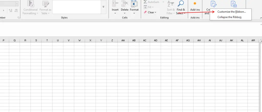
- Go to the Ribbon at the top of Excel.
- Right-click in an empty space or on any tab, and select Customize the Ribbon (or Customize Quick Access Toolbar if you prefer adding it there).
- This will open the Excel Options dialog box.
2. Find the Camera Tool
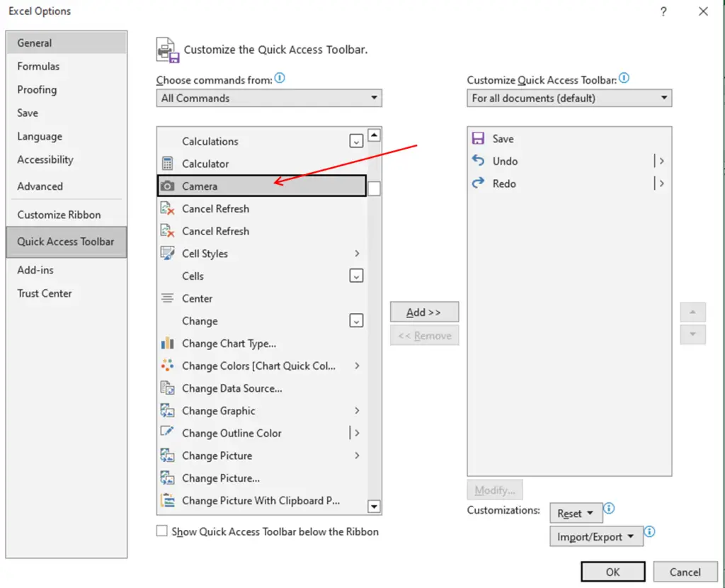
- In the Excel Options dialog, look for the Choose commands from dropdown.
- Select All Commands from the dropdown list.
- Scroll down through the commands until you see Camera (it’s usually alphabetical).
3. Add It to Your Toolbar
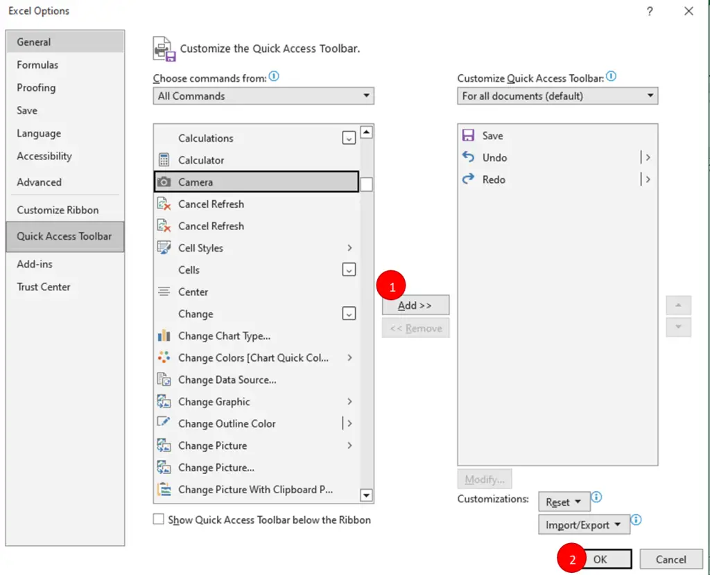
- Select Camera from the list.
- Click Add (to move it into the “Customize Quick Access Toolbar” or your chosen Ribbon group).
- Click OK to confirm.
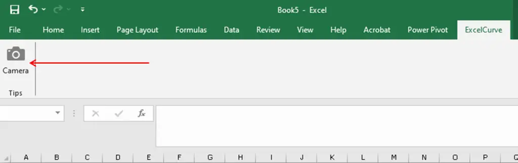
4. Confirm the Camera Icon
- You should now see a Camera icon in your Quick Access Toolbar or Ribbon.
- It might look like a tiny camera or some variation of it depending on your Excel version.
Taking Your First Snapshot
Now that you’ve enabled the Camera Tool, it’s time to see it in action:
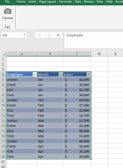
1. Select the Range You Want to Capture
- Highlight the cells or chart you want to monitor.
- I like to group logical data (e.g., monthly sales figures, inventory counts) so my snapshots are concise.
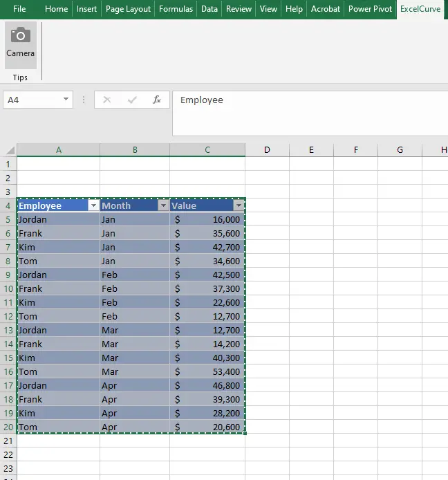
2. Click the Camera Icon
- With the cells still selected, click the Camera icon in your toolbar.
- Your cursor will now transform into a small + (plus sign) with a camera symbol.
3. Paste the Snapshot
- Navigate to the location where you want your live snapshot displayed (it could be a different worksheet or even a different workbook).
- Click once to “paste” your snapshot.
- You’ll see a rectangular image of the selected cells appear.
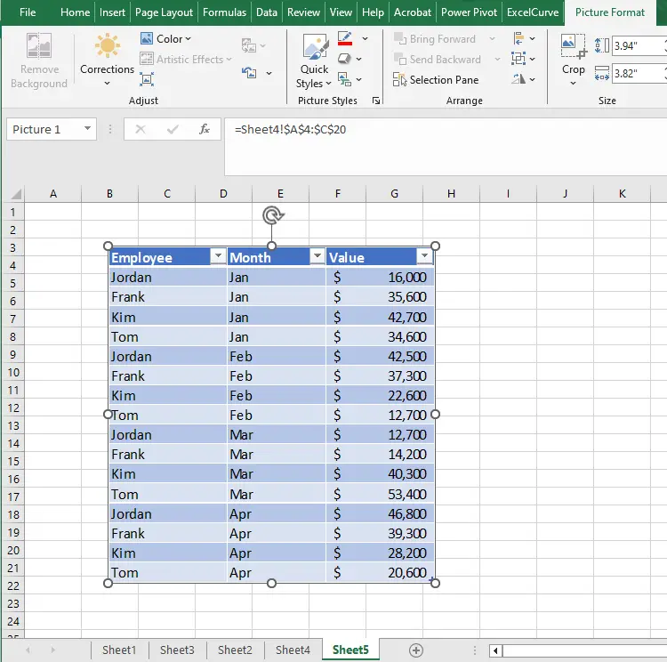
4. Resize and Move
- You can drag the corners of the snapshot to resize it.
- Position it wherever it’s most convenient on your sheet.
- It behaves like a regular image, except it remains dynamically linked to the original cells.
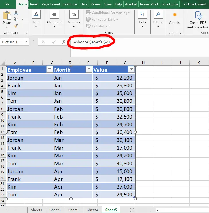
Real-Time Updates in Action
Here’s the best part: if you go back to the original range and update any value, the snapshot changes instantly. Let’s say you adjust a monthly sales figure from 500 to 550:
- Change the data in the source cells.
- Watch the snapshot update automatically in your dashboard sheet.
It’s a small thrill the first time you watch the numbers morph in real time without any extra steps required.
Pro Tips and Use Cases
- Dashboards: Keep essential metrics visible at all times, even if they’re spread across various sheets.
- Printing: If you need a single page with summary stats, you can “pin” different snapshots together, making printing quick and organized.
- Collaboration: When sending a workbook to a colleague, they can glance at the Camera snapshots for an at-a-glance view, rather than digging through multiple sheets.
Common Troubleshooting
- Disappearing Snapshot: If you accidentally delete the source range or drastically change the layout, your snapshot might behave oddly. Always keep the source range intact.
- Low Resolution: Depending on how much you resize the image, text can appear blurry. If this happens, consider using multiple snapshots of smaller ranges.
My Workflow, Transformed
Since discovering this feature, I’ve streamlined so many of my tasks in Excel. Instead of jumping from sheet to sheet to check up on a handful of KPIs, I now keep them all in a single sheet filled with dynamic snapshots. This one tiny button has fundamentally changed how I interact with my data—making it easier to stay on top of updates and focus on what really matters.
If you haven’t tried the Camera Tool yet, I can’t recommend it enough. Whether you’re a casual user or a power user, having these dynamic “windows” into your data can save time, reduce errors, and keep your focus on the bigger picture. Give it a shot (pun intended)—you may find it just as useful as I do.
If you like this one and are interested in learning countless additional tricks that are just as helpful, you should checkout the Excel Essentials course by our partner XelPlus.
Have a favorite hidden Excel feature of your own? Feel free to share your discoveries or any creative uses of the Camera Tool in the comments below!