
If you need to apply the accounting number format in Excel, it is very similar to the Currency format and can be applied to any list of numbers where needed. The difference between the Accounting format and the Currency format is that the Accounting format will add the dollar sign on the far left and will also put a dash where the number equals zero (instead of the zero digit).
So let’s use a simple to follow example to show how to apply the accounting number format in Excel step by step.
How to Simultaneously Apply Accounting Number Format in Excel
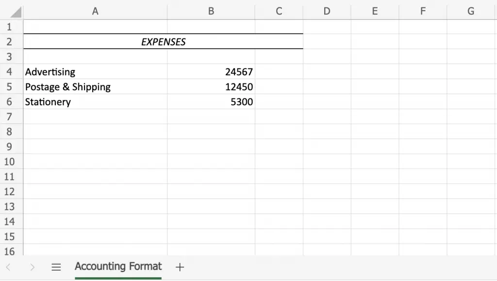
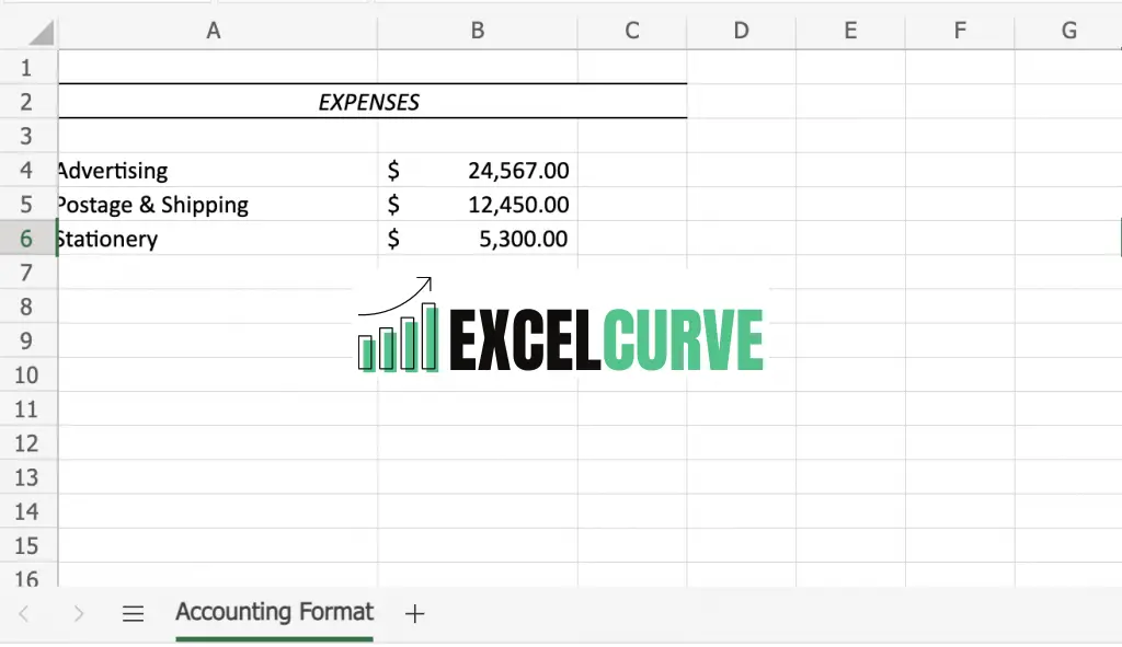
In this example, an accountant from our completely made up Accounting firm, XYZ Accountants is compiling a spreadsheet for their client, detailing the total expenses for the current financial year as shown below.
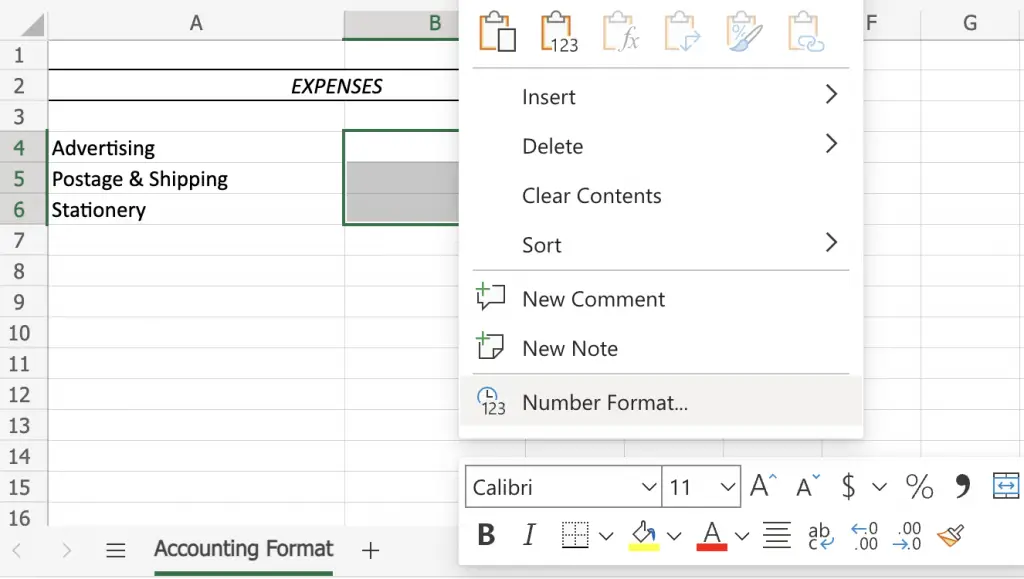
- To apply the Accounting format, select the range for the data you wish to convert, right click and select Number Format.
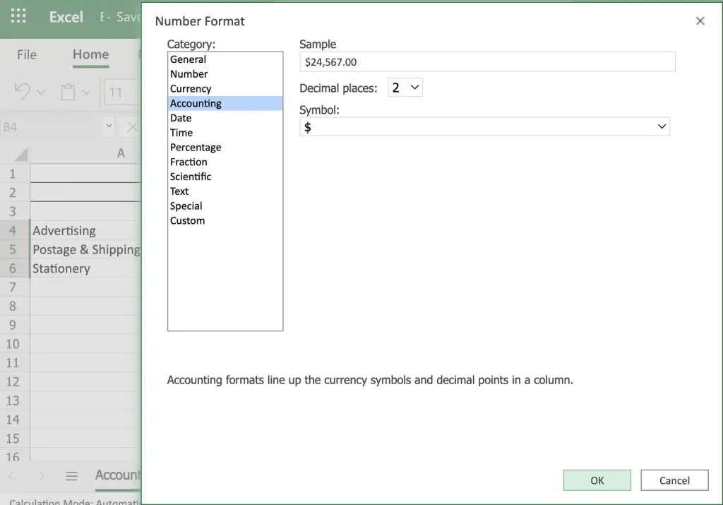
2. In the Number Format selection box, choose Accounting from the category list. Choose the decimal places and currency symbol you wish to work with and then press OK.
3. The Accounting format is now applied and all the currency symbols and decimal points will now be lined up directly beneath each other.
Conclusion
So that’s all there is to it when applying the Accounting number format in Excel. You can can use the Accounting format when compiling any sort of financial statements or balance sheets when performing Accountancy related functions.