
When is the new dynamic-array formula better, and when should you stick with the old drag-and-drop UI?
The PIVOTBY function is a recent addition to Excel, designed to offer a formula-based alternative to traditional PivotTables. As a new pivotby function and excel function, it enables users to create dynamic, real-time summaries directly in the worksheet. PIVOTBY is part of a set of new pivotby functions, including GROUPBY, that allow for flexible and interactive reporting through formulas.
Feature | PIVOTBY (Formula) | PivotTable (UI) |
|---|---|---|
Definition | Formula that summarizes data by grouping and aggregating (using row_fields, col_fields, values, and function arguments as its core syntax) | Drag-and-drop table for summarizing data |
Output | Dynamic array, updates automatically | Static table, requires refresh |
Use case | Real-time, formula-driven reports; advanced customizations | Quick summaries, easy UI |
In summary, the key difference between PIVOTBY and traditional PivotTables lies in PIVOTBY’s formula-driven approach and its use of explicit arguments—row_fields, col_fields, values, and function—to structure and aggregate data. This makes the new pivotby function especially useful for dynamic, customizable reports, while PivotTables remain ideal for quick, UI-based summaries.
TL;DR
PIVOTBY is a single formula that spills a pivot-style summary right in the grid. A classic is an object with its own Field List, slicers, and refresh cycle. Use PIVOTBY for formula-driven dashboards; use PivotTables for slicers and huge datasets.
PIVOTBY | PivotTable | |
|---|---|---|
Definition | Dynamic-array function that groups rows/columns and aggregates a value field. | Interactive object inserted via Insert → PivotTable. |
Introduced | Microsoft 365 public release (2024) [Microsoft Support] | Excel ’97, continually upgraded [Microsoft Support] |
Output | Spill range that auto-expands and recalculates. | PivotTable object stored in a PivotCache; refresh on demand. |
UI | Formula bar only (=PIVOTBY(RowField,ColField,ValueRange,AGG)) | Drag fields in a pane; slicers, timelines, PivotCharts. |
1 | Introduction to PivotBy and PivotTables
The Excel PivotBy function and classic PivotTables are both essential tools for data summarization and analysis, but they approach the task in different ways. The PivotBy function is a new dynamic array function in Excel 365 that lets you create a pivot-style summary directly in the worksheet using a single formula. With the excel pivotby function, you can group data, aggregate values, and generate a dynamic report that automatically expands as your source data grows—making it ideal for modern, formula-driven workflows.
On the other hand, PivotTables have long been the go-to feature in Excel for summarizing and analyzing large datasets. A PivotTable is an interactive object that you create through Excel’s interface, allowing you to drag and drop fields to quickly build reports and extract insights from your data. PivotTables are especially powerful for users who prefer a visual approach to data analysis and need to work with large or complex datasets.
Understanding the basics of both the PivotBy function and PivotTables is key to choosing the right tool for your needs. While the PivotBy function offers a formula-based, dynamic array approach to data summarization, PivotTables provide a robust, object-based solution for exploring and reporting on data in Excel.
2 | When to Choose Which
Deciding whether to use the PivotBy function or a classic PivotTable depends on the specific requirements of your analysis. The excel pivotby function shines when you need to create dynamic, formula-driven reports that automatically update as your data changes. It’s particularly effective for analyzing data across multiple columns and row fields, and for scenarios where you want to apply multiple aggregations—such as sum, average, or count—using a single, flexible formula.
If your goal is to analyze data with multiple aggregations and you value the ability to customize your report layout directly in the worksheet, the PivotBy function is a strong choice. It’s also ideal for dashboards that need to expand or contract as new data is added, thanks to its dynamic array capabilities.
However, if you’re working with very large datasets or need to create reports with a fixed layout and advanced formatting, PivotTables may be the better option. PivotTables are designed to handle large volumes of data efficiently and offer a familiar, drag-and-drop interface for building reports. They also provide built-in features for formatting, sorting, and filtering, making it easy to create polished, presentation-ready summaries.
In summary, use the PivotBy function for flexible, formula-based reports with multiple columns and aggregations, and choose PivotTables when you need robust formatting, compatibility with large datasets, and a user-friendly interface for creating and managing your reports.
3 | Hands-On Comparison (Sales Example)
To see the differences between the PivotBy function and PivotTables in action, let’s walk through a simple sales example. Imagine you have a dataset containing sales data with columns for region, product, and sales amount. Your goal is to create a report that displays the total sales by region and product.
Using the pivotby function, you can quickly generate a dynamic array that summarizes your data. For example, the following formula groups your sales data by region and product, calculating the total sales for each combination:
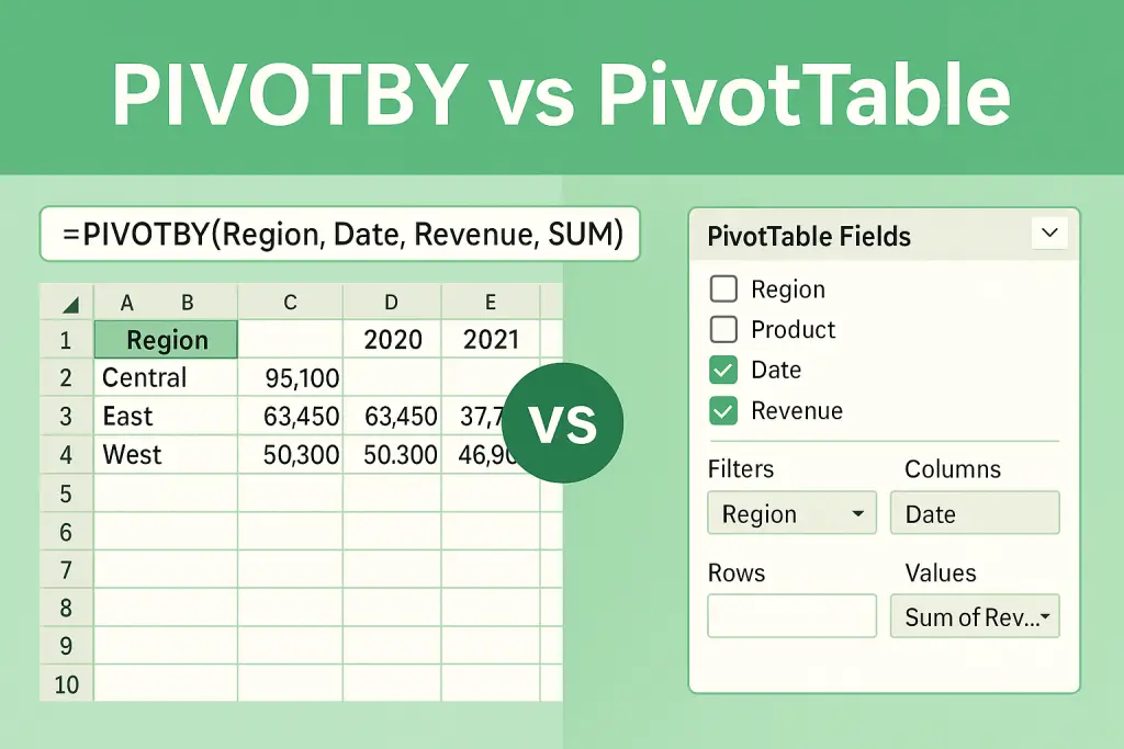
=PIVOTBY(SalesData[Region], SalesData[Product], SalesData[Revenue], SUM)
This formula instantly creates a matrix of total sales, with regions as rows and products as columns. The dynamic array automatically expands as new data is added, ensuring your report stays up to date.
Alternatively, you can use a PivotTable to achieve the same results. Simply select your sales data, insert a PivotTable, and drag the region field to the rows area, the product field to the columns area, and the sales amount to the values area. The PivotTable will display the total sales for each region and product, with built-in options for formatting and layout.
While both tools can create the same summary, the PivotBy function offers a more dynamic, formula-driven approach, while PivotTables provide a familiar, interactive interface with advanced formatting options. Choose the method that best fits your workflow and reporting needs.
2 | When to Choose Which
Use-case | Go PIVOTBY if … | Stick to PivotTable if … |
|---|---|---|
Quick one-off summaries | You prefer typing formulas. The groupby function is another option for summarizing data, and it requires fewer arguments than PIVOTBY for simple summaries. | You’d rather drag fields—no formulas. |
Auto-expanding dashboards | Spill ranges resize with new rows automatically. | You need slicers or PivotCharts. |
Model transparency / audits | Formula shows logic in the bar. You can use different functions for aggregation, such as calculating the average and count simultaneously, and the groupby function can also be used for data grouping and summarization. | Stakeholders expect the familiar object. |
Very large data (>100 k rows) | Works, but full recalc each sheet change. | PivotCache is more efficient; refresh on demand. |
3 | Hands-On Comparison (Sales Example)
3.1 Data Setup
Table name SalesData with columns Date, Region, Product, Units, Revenue (same as our Dynamic Arrays guide).
3.2 PIVOTBY Formula
=PIVOTBY(SalesData[Region], SalesData[Product], SalesData[Revenue], SUM)
Spills a matrix of revenue by Region × Product—instantly updates when new rows are added.
3.3 Classic PivotTable
- Select any cell in SalesData
- Insert → PivotTable → place on new sheet
- In the PivotTable Fields pane, drag Region to Rows, Product to Columns, Revenue to Values (Sum). You can select and arrange PivotTable fields here to customize your analysis. Field headers can also be customized for clarity, especially when aggregating multiple columns. You can sort rows and columns to organize your report layout as needed.
- (Optional) Insert a slicer for Date to make filtering data easier. You can also use the filter dropdowns in the PivotTable to filter data. For visual analysis, consider adding pivot charts to your report.
3.4 Side-by-Side Outputs
PIVOTBY spill | PivotTable object | |
|---|---|---|
Auto-expands? | ✓ (new products add new columns and as many cells as needed) | Only after Refresh |
Grand totals | Add manually or via EXPAND; grand total row can be customized | Built-in toggles for grand total and grand total row |
Row totals / Column totals | Customizable with total_depth and relative_to; row totals, row total, column totals, and total rows can be shown or hidden | Built-in options for row totals, column totals, and total rows |
Column fields / Row and column fields | Column fields, row and column fields, and column labels can be customized for clarity | Column fields and row and column fields are set via drag-and-drop; column labels can be sorted |
Formats | Formats for headers, totals, and data can be adjusted with formatting functions | Multiple built-in formats and styles for all areas |
Slicers | ✗ | ✓ |
Referencing in charts | Use A2# or TAKE() | Use PivotTable structured refs |
Same column aggregations | Multiple aggregations on the same column using HSTACK or by placing the same column in different value areas | Add the same column multiple times to Values area for different aggregations |
Default behavior | Totals and formatting are applied by default based on function arguments; spills into as many cells as needed | Totals and formats are enabled by default but can be toggled |
Noticeable difference | PIVOTBY spills results into as many cells, allows flexible use of the same column for multiple aggregations, and offers formula-based customization; PivotTable provides a user interface for quick formatting and built-in grand total row |
4 | Data Sources and Compatibility
Both the PivotBy function and PivotTables are versatile when it comes to handling different data sources. You can use the excel pivotby function with Excel tables, structured ranges, and even data imported from external sources. However, it’s important to note that the PivotBy function is only available in Excel 365 and the latest versions of Excel, making it inaccessible in older versions.
PivotTables, on the other hand, are available in all versions of Excel, from Excel 97 onwards. They can connect to a wide range of data sources, including Excel tables, ranges, databases, and online data feeds. This makes PivotTables a reliable choice for users who need compatibility across different versions of Excel or who work with large datasets from multiple sources.
When working with large datasets, consider the performance and compatibility of each tool. The PivotBy function is optimized for dynamic array calculations in Excel 365, while PivotTables are designed to efficiently summarize and analyze data from a variety of sources. For best results, choose the tool that matches your version of Excel and the size and complexity of your data sources.
5 | Conditional Formatting and Customization
Customizing your reports is easy with both the PivotBy function and PivotTables, but each tool offers different approaches to conditional formatting and layout. With the pivotby function, you can use Excel’s built-in conditional formatting tools or create custom rules using formulas. This allows you to highlight specific rows, columns, or values based on your own criteria, making your dynamic array reports more insightful and visually appealing.
You can also use the pivotby function to group rows and columns, and to create grand totals or subtotals by combining it with other dynamic array functions like EXPAND or VSTACK. For advanced users, the PivotBy function supports custom lambda functions, enabling you to define your own aggregation logic for even more tailored reports.
PivotTables, meanwhile, offer a range of built-in formatting and customization options accessible from the design tab. You can quickly apply conditional formatting, change the report layout, and add grand totals or subtotals with just a few clicks. PivotTables also make it easy to group data, sort columns, and format your report for presentation.
Whether you prefer the formula-driven flexibility of the PivotBy function or the user-friendly customization features of PivotTables, both tools provide powerful options for creating polished, informative reports in Excel. Experiment with each approach to find the best fit for your data and reporting style.
4 | Performance Notes
- Recalc cost: PIVOTBY re-executes on each workbook recalculation; PivotTables recalc only on Refresh.
- Memory: PivotTables compress data in a PivotCache.
- Volatility: PIVOTBY is semi-volatile—recalc triggers only when referenced ranges change.
5 | Limitations & Work-Arounds
Limitation | Work-around |
|---|---|
One aggregation at a time | Nest multiple PIVOTBY formulas side-by-side or use a PivotTable. |
No grand totals row/column | Wrap with EXPAND or VSTACK a manual total. |
No slicers | Wrap PIVOTBY in FILTER(), or use classic PivotTables. |
Not in Excel 2019/2016 | Requires Microsoft 365 or Excel 2024 perpetual. |
6 | Practical Recommendations
- Formula-centric dashboards: use PIVOTBY. Generating reports with excel formulas like PIVOTBY allows for dynamic analysis of aggregated data, making it easier to summarize and present complex information.
- Reports for non-Excel power users: use PivotTables. Excel’s built-in PivotTables provide robust data summarization and reporting capabilities, especially when working with multiple data columns and field headers for clarity.
- Power Query / Power Pivot data models: PivotTables still reign.
- Hybrid: quick PIVOTBY checks inside prep sheet → polished PivotTable for presentation.
Further Reading
- Microsoft Support – PIVOTBY function
- Microsoft Support – Create a PivotTable
- ExcelCurve – Dynamic Arrays Demystified
- Excel training resources and tutorials
Last updated: May 9, 2025