

There are situations in Excel where you would want to count values in one column based on criteria in another column or columns. For example, you may want to find out from your dataset how many manufacturers of different products are based in certain regions of the country.
Some of the ways of counting values in one column based on criteria in another column(s) are:
- Employ PivotTable
- Apply the COUNTIF function
- Make use of the COUNTIFS function
- Use the SUMPRODUCT function
In this tutorial, we explore these ways and demonstrate exactly how they can be used in different situations.
1. Employ the PivotTable
A PivotTable can be used to summarise data and show the count of values in a column based on criteria in another column(s).
We create the PivotTable by doing the following:
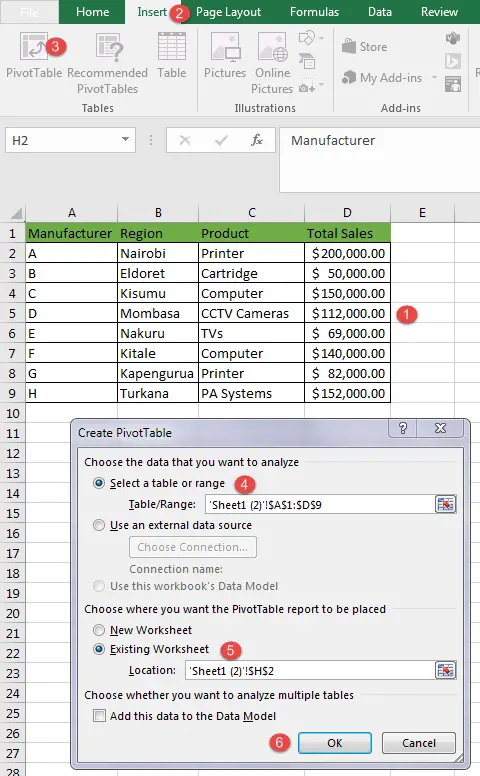
Step 1 – Select the dataset you want to work with. In the example below it is range $A$1:$D$9.
Step 2 – On the Excel Ribbon, click the Insert tab.
Step 3 – Click on the PivotTable command button.
Step 4 – Ensure that Select a table or range option is selected in the Create PivotTable dialog box and that the right data range is selected.
Step 5 – Select the Existing Worksheet option in choosing where you want the PivotTable to be placed. Click in the Location box and select an empty cell.
Step 6 – Press OK.
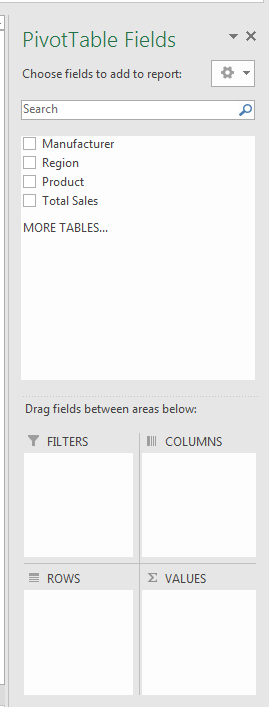
After pressing OK, the PivotTable fields will appear on the right of the Excel window.
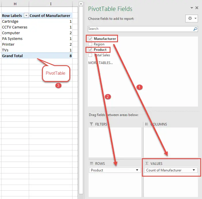
In our example, to find out the number of manufacturers who make the different products, drag the Manufacturer field into the VALUES box below and the Products field into the ROWS box.
We will get a PivotTable showing the number of manufacturers that produce different products as shown below:
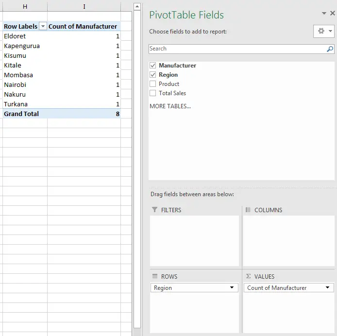
If we want to find out how many manufacturers are located in each region, we need to untick the Product field and select the Region field. The PivotTable will adjust accordingly to show the count of manufacturers in the different regions as shown below:
2. Apply the COUNTIF function
We can use the COUNTIF function to count values in one column that meet the criteria in another column.
In the following example, we want to find out how many manufacturers make printers.
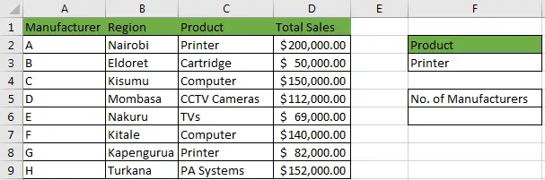
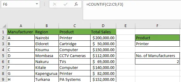
To get how many manufacturers make printers, we enter the following formula =COUNTIF(C2:C9,F3) in cell F6.
The data range C2:C9 is where the counting takes place. Cell F9 contains the criteria that is applied, which in this case is Printer.
The correct count of 2 manufacturers is returned as shown below:
See Also: Excel COUNTIF Partial Match (With Examples)
3. Make use of the COUNTIFS function
We make use of the COUNTIFS when we want to get the count of values in a column based on multiple criteria.
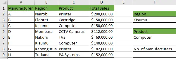
Suppose we want to find out how many computer manufacturers are based in Kisumu city, based on the following dataset.
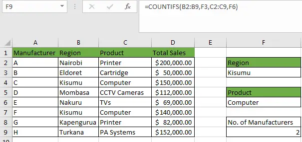
We will need to enter the formula =COUNTIFS(B2:B9,F3,C2:C9,F6) in cell F9. When we press the Enter key, we will get the correct count of 2 computer manufacturers based in Kisumu city as shown below:
4. Use the SUMPRODUCT FUNCTION
We can also use the SUMPRODUCT function to count values in one column that meet the criteria in another column.
For example, we may want to find out how many manufacturers make printers based on the following dataset:
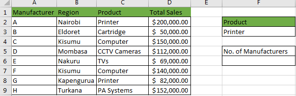
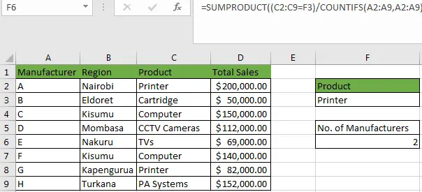
To get the correct count we need to input the formula =SUMPRODUCT((C2:C9=F3)/COUNTIFS(A2:A9,A2:A9)) in cell F6.
The data range A2:A9 is where the counting takes place. Range C2:C9 is the criteria range. In this case, the criteria is Printer, and it is referred to in cell F3.
When we press ENTER, we will get the correct count of 2 printer manufacturers as shown below:
Conclusion
In this tutorial, we have looked at different formulas to count values in a column that meet conditions or criteria in another column(s). You can use one or all of the ways depending on your situation and use case in Excel.