

The COUNTIF function counts the number of cells within a given data range that meet specified criteria or conditions. COUNTIF can be used to find partial matches in Excel as well.
The COUNTIF function can also return the number of cells that contain text values that partially match the criteria value.
We will use the following dataset to demonstrate how the COUNTIF function can be used to count cells that have values that partially match the criteria value:
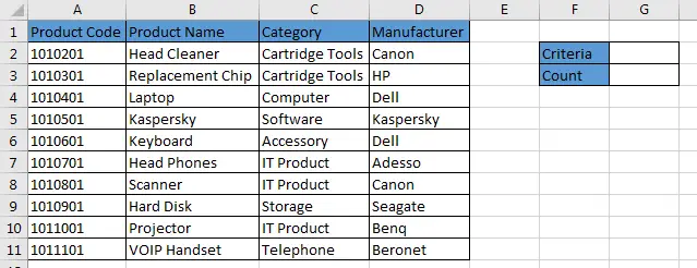
The dataset shows the product details of 11 products.
Our dataset is small for demonstration purposes but in a practical situation, you will normally work with very large datasets.
Use of wildcards in Excel
Wildcards play such an important role when we use the COUNTIF function to return the count of partial matches in an Excel workbook. Wildcards are the special characters that can take the place of any character.
There are only three wildcard characters that are used in Excel:
- ? (Question mark). It takes the place of only one character. For instance Cor? could return Cork or Core.
- * (Asterisk). It takes the place of one or more characters. For instance, Con* could return Conman, Contrary, or Contract.
- ~ (tilde). It is used to show the question mark (?) and asterisk (*) characters. For instance Cor~? would return Cor? and Con~* would return Con*.
The most commonly used wildcard characters in Excel are the Question mark (?) and the asterisk (*).
It is important to note that these wildcard characters work only with text values and not numbers.
Examples of Uses of COUNTIF in Partial match
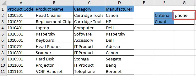
Example 1 – How to return the count of Product Category names that contain the word phone:
Step 1 – Enter the word “phone” in cell G2. This is the criteria value:
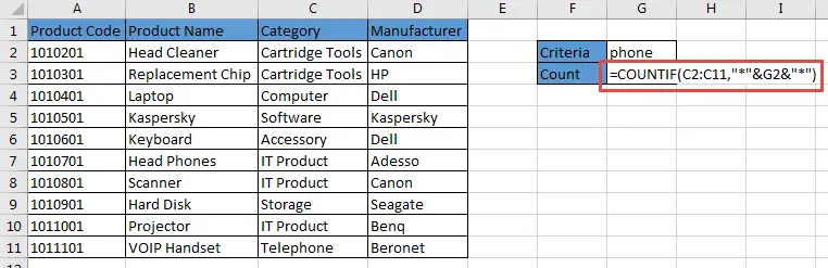
Step 2 – Enter the formula =COUNTIF(C2:C11,”*”&G2&”*”) in cell G3:
Step 3 – Press the Enter key:
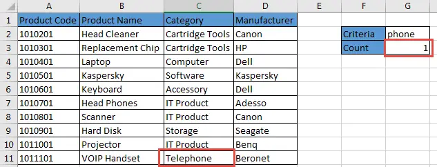
The COUNTIF function returned the value of 1 meaning there is only one partial match in the data range, which in this case is the Telephone Category.
Explanation of the =COUNTIF(C2:C11,”*”&G2&”*”) formula:
The COUNTIF function has the two arguments:
- C2:C11 is the data range in which the function will look for partial matches.
- “*”&G2&”*” is the criteria or condition for the partial match. See that cell G2 which contains the criteria value is flanked by asterisks (*) on both sides. Also, note that the asterisks are in double-quotes and joined to cell G2 using the concatenating character (&).
Changing Criteria
We can change the criteria value in cell G2 and the COUNTIF function will return the correct count of partial matches. For example, let’s change the criteria value to Cartridge:
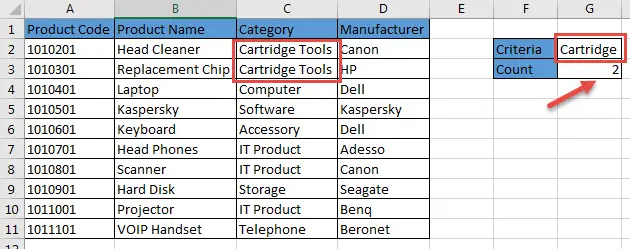
The count has been updated accordingly.
COUNTIFS function
The COUNTIF function we have so far used can only return the number of cells that meet one condition. If we want to return the count of cells that meet more than one condition, we have to use the COUNTIFS function.
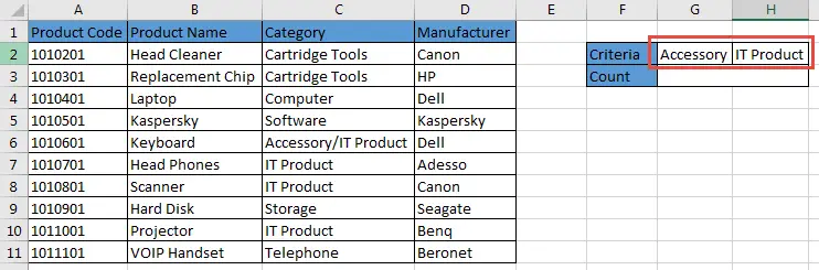
Example 2 – How to return the count of Product Category names that contain the words Accessory and Product:
Step 1- Enter the word Accessory in cell G2 and the word Product in cell H2:
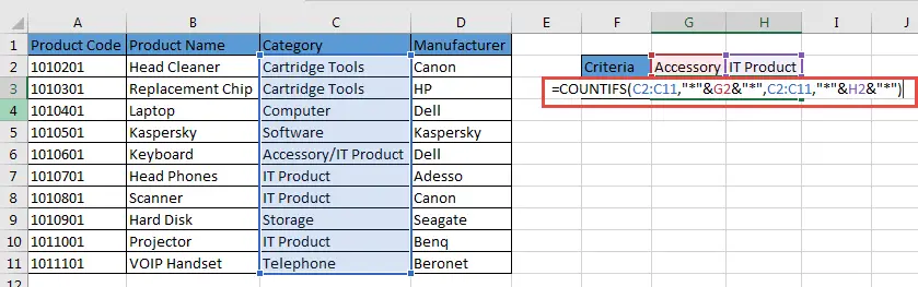
Step 2 – Enter the formula =COUNTIFS(C2:C11,”*”&G2&”*”,C2:C11,”*”&H2&”*”) in cell G2:
Step 3 – Press the Enter key:
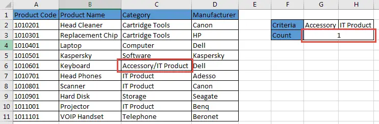
We get the count of 1 because only the Accessory/IT Product Category meets both conditions.
Explanation of the =COUNTIFS(C2:C11,”*”&G2&”*”,C2:C11,”*”&H2&”*”) formula:
This formula has 2 conditions for the partial matches: “*”&G2&”*” and “*”&H2&”*”.
The COUNTIFS function looks for the partial matches in the same data range C2:C11 for both conditions or criteria.
Conclusion
In this tutorial, we have looked at how one can use the COUNTIF and COUNTIFS functions to return the count of cells that contain values that partially meet certain conditions.
Thanks for reading! We’d love to hear from you—what Excel challenges are you facing? Drop a comment or let us know what tutorials you’d like to see next! Finally, be sure to check out the Excel courses to help master your Excel skills.