

You are given an Excel file dataset to work on and you discover that it has so many unnecessary parentheses. How do you remove parentheses in Excel? You may decide to remove them one by one by selecting and deleting them using the delete key, but this would be tedious and quite time-consuming, especially if you have a large dataset.
In this tutorial, we look at the following 4 effective ways that you can use to easily remove parentheses in Excel:
- Use the Find and Replace feature.
- Use the SUBSTITUTE function.
- Use Excel VBA code.
- Use a combination of LEFT and FIND functions.
We will use the following dataset to demonstrate how each of the methods can be applied.

1. Use the Find and Replace feature to remove parentheses
This method is the easiest and most commonly used by many people. The Find and Replace feature works by replacing all the parentheses in the selected dataset with blanks.
To apply this method, we do the following:
Step 1 – Select the dataset from which you want to remove parentheses.
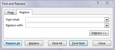
Step 2 – Press the Ctrl key and then the H key to launch the following Find and Replace dialog box.
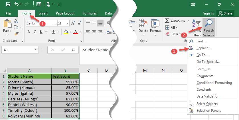
We can also open the Find and Replace dialog by navigating to Home>>Find & Select>>Replace as shown below:
Step 3 – To remove the starting or opening parenthesis, type “(“ in the Find what input box and leave the Replace with input box blank as shown below:

Step 4 – Click the Replace All button to remove all the opening parentheses from the dataset.
The following dialog box will pop up showing that the operation has been successful:

Click OK on the dialog box and the dataset will now appear as follows:

Step 5 – Repeat steps 2, 3, and 4 to remove all the closing parentheses. In step 3 ensure that you type “)” in the Find what input box.
All parentheses will now be removed and the dataset will appear as follows:

2. Use the SUBSTITUTE function
We use this method if we prefer to leave the original dataset as it is.
The SUBSTITUTE function is used to substitute a set of characters for another.
Do the following to remove all the parentheses from your dataset using the SUBSTITUTE function:
Step 1- Select the dataset from which you want to remove the parentheses.
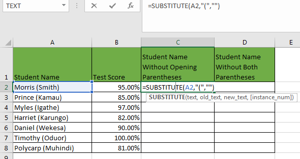
Step 2 – In cell C2 enter the formula =SUBSTITUTE(A2,”(“,””) as shown below:
Step 3 – Press the Enter key and use the Fill handle to copy the formula down to all the cells in Column C. All the opening parentheses will be removed from range C2:C8 as shown below:

Step 4 – In cell D2 enter the formula =SUBSTITUTE(C2,”)”,””) as shown below:

Step 5 – Press the Enter key and use the Fill handle to copy the formula down to all the cells in Column D. All the closing parentheses will be removed from range D2:D8 as shown below:
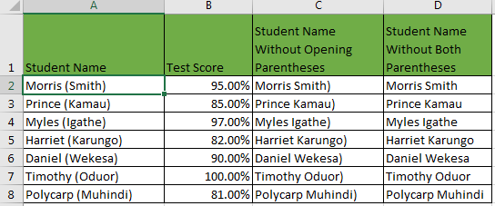
Step 6 – To retain the original values in Column A, copy the contents of Column D and paste them into Column C by value (CTRL+Alt+V). Then delete Column D and your dataset will look as follows:

3. Use Excel VBA macro
In the previous methods, we had to remove one parenthesis at a time but with VBA code, we can remove all the parentheses at once. This saves time and effort.
Follow the following steps to remove parentheses from your dataset using VBA code:
Step 1 – Press Alt+F11 and copy the following VBA code into a module.
Sub RemoveParentheses()
Cells.Select
Selection.Replace What:=”(“, Replacement:=””, LookAt:=xlPart, _
SearchOrder:=xlByRows, MatchCase:=False, SearchFormat:=False, _ ReplaceFormat:=False
Selection.Replace What:=”)”, Replacement:=””, LookAt:=xlPart, _
SearchOrder:=xlByRows, MatchCase:=False, SearchFormat:=False, _ ReplaceFormat:=False
End Sub
Step 2 – Select the dataset you want to remove the parentheses from.
Step 3 – Press Alt+F8 to open the macro dialog box. Select and then run the macro.
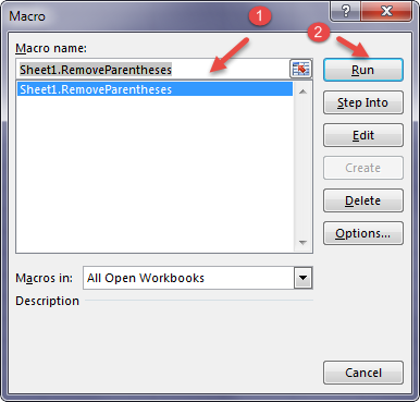
The macro will remove all parentheses from your dataset at once.
4. Use a combination of LEFT and FIND functions.
By using the combination of LEFT and FIND functions, we can remove parentheses from any dataset.
We use the LEFT function to return a specified number of characters from the start of a text string. The FIND function is case-sensitive and returns the starting position of one text string within another text string.
Follow these steps to apply these functions in removing parentheses:
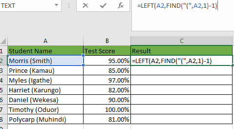
Step 1 – In cell C2 enter the formula =LEFT(A2,FIND(“(“,A2,1)-1) as shown below:
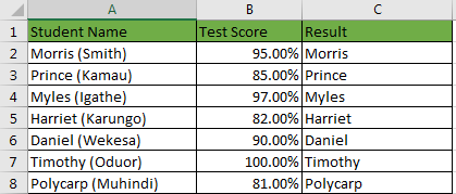
Step 2 – Using the Fill handle, copy the formula down to the rest of the cells in Column C.
Explanation of the formula:
In cell C2, the FIND function pinpoints the position number of the opening parenthesis beginning from the start and returns the number 8.
We subtract 1 from the 8 so that the LEFT function retains only 7 characters starting from the left, and this returns Morris. The same process applies down Column C.
Conclusion
In this tutorial, we have looked at four methods of removing parentheses in Excel. You can apply any or all of the methods depending on what you are working on.