

The VLOOKUP (Vertical Lookup) function is one of the powerful Excel functions that is used widely by many people every day. It is normally used to look for a single matching value in the first column of a table and return a single value in the same row from a different specified column.
However, in combination with COUNTIF, INDIRECT, and ROW functions, the VLOOKUP function can be used to return multiple values vertically.
In this tutorial, we will demonstrate how this can be achieved.
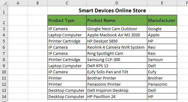
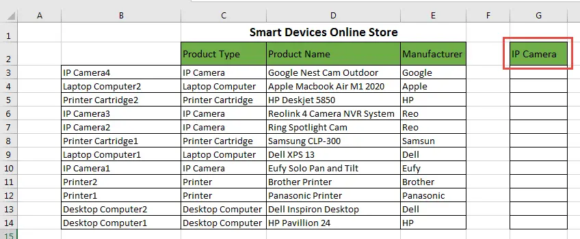
We will use the following dataset to explain and demonstrate how we can use the VLOOKUP function to look for a particular matching value and then return all the values based on that particular value.
You can reproduce the dataset in an Excel file exactly as it appears below so that you follow the tutorial.
Steps to Vertically Returning Multiple Values in Excel using the VLOOKUP Function
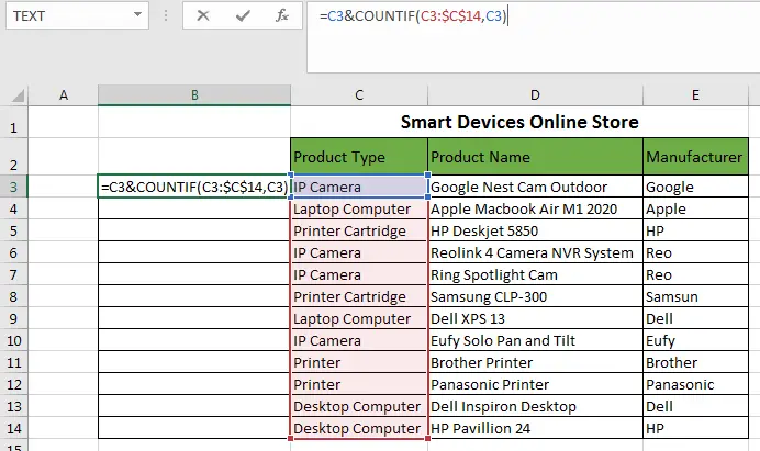
Step 1 – Move to Column B which we shall make a helper column.
Step 2 – Enter the formula =C3&COUNTIF(C3:$C$14,C3) in cell B3 as follows:
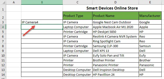
When you press the Enter key, the following result will appear:
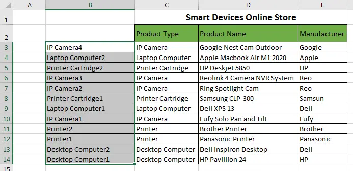
Step 3– Click on the Fill Handle and drag it down to the last cell. You will then see a list of Product Types with their serial numbers, for example, Desktop Computer1, Desktop Computer2:
Step 4 – Move to Column G and key in the name of the Product Type that you want to look up as the Column Header.
In the following example, I have keyed in IP Camera in cell G2:
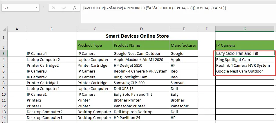
Step 4 – Enter the formula =VLOOKUP(G2&ROW(A1:INDIRECT(“A”&COUNTIF(C3:C14,G2))),B3:E14,3,FALSE) in cell F3 and then press the Enter key if you are using Office 365. If not, select many cells first before entering the formula, and once you have entered the formula press CTRL+SHIFT+ENTER.
You will see the following multiple values which are the names of IP Cameras:
When you change the lookup value in cell G2, you will get different values in the column. For example, if you change the lookup value to Laptop Computer, you will get a list of the names of laptop computers in the dataset.
Explanation of the formula
=VLOOKUP(G2&ROW(A1:INDIRECT(“A”&COUNTIF(C3:C14,G2))),B3:E14,3,FALSE)
G2 is the cell that has the lookup value, which in this case is IP Camera, and can be changed to any of the other Product Types depending on which Product Names you want to be returned.
Range C3:C14 is the lookup range and the first column of the dataset.
Range B3:E14 is the table array together with the helper column B.
3 is the column index number, representing the column that has the data we want to be returned, in this case, Product Name.
The COUNTIF function is innermost in the formula and it computes how many cells in the lookup range C3:C4 contain the lookup value in cell G2. In this case, it returns the value of 4.
The value 4 is passed to the INDIRECT function leading to read INDIRECT(“A”&4), yielding the cell reference A4.
The ROW function now gets the argument of range A1:A4 and becomes ROW(A1:A4).
The ROW function returns the array {1,2,3,4}.
The value in cell G2 is then concatenated with the array returned by the ROW function, resulting in another array {IP Camera1, IP Camera2, IP Camera3, IP Camera4}.
The formula =VLOOKUP(G2&ROW(A1:INDIRECT(“A”&COUNTIF(C3:C14,G2))),B3:E14,3,FALSE) now becomes =VLOOKUP({IP Camera1, IP Camera2, IP Camera3, IP Camera4},B3:E14,3,FALSE).
Each value of the array {IP Camera1, IP Camera2, IP Camera3, IP Camera4} is looked for in the lookup column B and the corresponding Product Name in Column 3 is returned and we get a list of the Product Names.
Conclusion
In this tutorial, we have shown how the VLOOKUP function together with the COUNTIF, INDIRECT, and ROW functions can be used to extract multiple values vertically from a dataset.